Amevoin K. Yves

1- Motivations

As a simple motivation, assume you have a sample of n observations from iids random variables with the Pareto distribution (I know the iid assumption is not obvious in practice, but let’s start with that). We know that the pareto distribution with shape parameter \(\alpha\) and strictly positive scale parameter \(x_m\) has a variance only for \(\alpha > 2\). Given \(\alpha\) in the previous mentioned interval, its expectation is equal to \(\frac{\alpha x_m}{\alpha - 1}\), and its variance is \(\frac{x_m^2\alpha}{(\alpha - 1)^2 (\alpha -2)}.\)

Assume we want to give a confidence interval of the mean (knowing \(\alpha > 2\)). We can directly think about using the central limit theorem (CLT) once we have our observations. But the central limit theorem uses two main things: (i) The empirical mean and (ii) asymptotic behavior. What if we fail to meet the asymptotic criteria (i.e few observations?). Moreover, we know that the CLT relies on the existence of moment of order 2, in our case for \(\alpha \in ]1, 2]\) our random variable does not have moment of order greater than 1. How can we build a confidence interval in that case?

2- Something more interesting

Let’s take a look in a case where \(\alpha = 3\) and \(x_m = 2\) with \(n\) taking values 5, 10, 15, 20, 25, 30, 35, 40, 45, 50… up to 100. We will have to rely on the inverse of the PDF to sample from the Pareto distribution. The PDF of the Pareto distribution is \(F(x) = \frac{\alpha x_m^\alpha}{x^{\alpha +1}}\) for \(x \in [x_m, \infty)\)

inverse_pareto <- function(u, alpha = 3, xm = 2){
  (u / (alpha * (xm ^ alpha))) ^ (-1/(alpha + 1))
}
#function for the mean of the pareto distribution
mean_pareto <- function(alpha = 3, xm = 2) alpha * xm / (alpha - 1)
#function for the variance of the pareto distribution
variance_pareto <- function(alpha = 3, xm = 2){
  (alpha * xm^2) / ((alpha -2) * (alpha -1)^2)
} 
confint <- function(vectr, variance, level = 0.05){
  low = mean(vectr) - qnorm(1 - level /2) * sqrt(variance / length(vectr) )
  high = mean(vectr) + qnorm(1 - level /2) * sqrt(variance / length(vectr) )

data.frame(low = low, high = high)
}

#apply the inverse of the Pareto PDF
n <- seq(5, 100, by = 5)
#now I replicate everything
U <- lapply(n, runif)
P <- lapply(U, inverse_pareto)

#The true variance (will help in computing CI's)
var <- variance_pareto()

truemean <- mean_pareto()

# cfit5 for confidence interval at "5%"
cfit5 <- lapply(P, function(x) confint(x, var))
cfit5 <- dplyr::bind_rows(cfit5)
cfit5$n <- n

Now Let’s plot the values of the confidence intervals we have found and the true value of the mean we know.

library(ggplot2)

plot_graph <- function(a_dat){
  ggplot(a_dat) +
    geom_segment(aes(x = low, y = n, xend = high, yend = n)) +
    geom_point(aes(x = low, y = n))+
    geom_point(aes(x = high, y = n))+
    geom_vline(xintercept = truemean, colour = "red")+
    scale_y_continuous(breaks = seq(0, 100, by = 5))+
    scale_x_continuous(breaks = seq(-1, 5, by = 0.5))+
    theme_light() +
    annotate("label", x = 3.5, y = 105, label = "True mean", colour = "red",
             fill = "pink")+
    annotate("segment", x = 3.05, xend = 3.1, y = 105, yend = 105, 
           arrow = arrow(ends = "first", length = unit(0.05, "inches")))
}

plot_graph(cfit5) +
    labs(x = "Length of 95%  confidence intervals, base on CLT",
         y = "Sample size")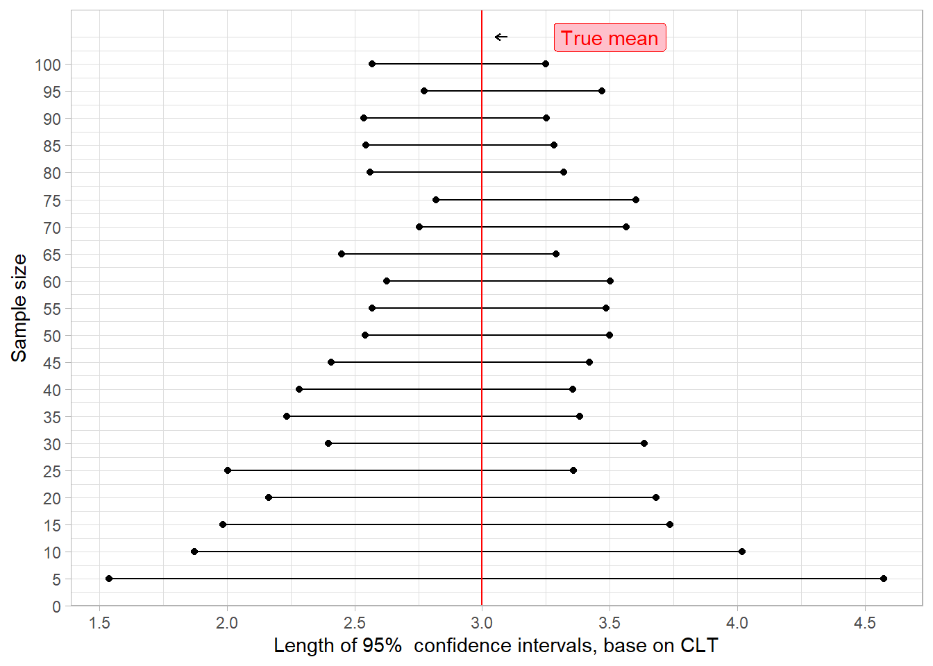

Clearly, we see that central limit theorem performs really bad in the case of small sample (with the known variance) with a so skewed distribution like the Pareto One. But we can even go further. Remember we computed confidence intervals of level 5%. What if we wanted something more precise? Let’s just take a look.

cfit <- lapply(P, function(x) confint(x, var, level = 0.001))
cfit <- dplyr::bind_rows(cfit)
cfit$n <- n

plot_graph(cfit)+
  labs(x = "Length of 99.999%  confidence intervals, base on CLT",
       y = "Sample size")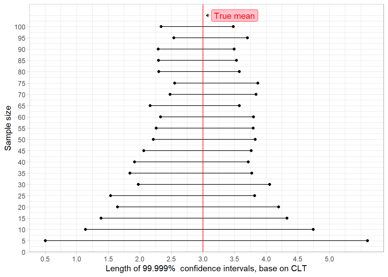

Okay, that sound less good. If you are having difficulties to compare both, here is a summary graph.

cfit5$level <- "5%"
cfit$level <- "0.1%"

bulk <- rbind(cfit, cfit5)

plot_graph(bulk)+
  facet_wrap(~level, nrow = 2) +
  labs(x = "Length of confidence intervals, base on CLT",
       y = "Sample size")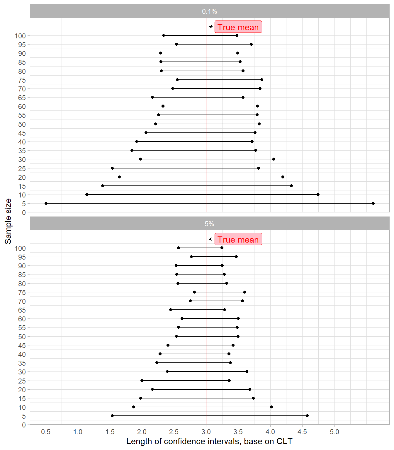

So Let’s think about another approach. What if we were able to build an estimator of our mean \(\mu_P\), called \(\widehat{E}(X_1^n)\), so that the equation

\[\begin{equation} \mathbb{P}\Big( |\widehat{E}(X_1^n) - \mu_P| > \sigma_P L \sqrt{\frac{1+\ln(1/\delta)}{n}} \Big) \leq \delta \mbox{ for } \delta \in [\delta_{min}, 1) \label{eqdet} \end{equation}\]

can hold for a large class \(P\) of distributions having moment of order 2 (noted \(\sigma_P^2)\)? \(L\) can be seen as a constant which does not depend on \(P\) and \(\delta_{min}\) as small as possible, say \(\delta_{min} \rightarrow 0\) exponentially when \(n \rightarrow \infty\). This can help us hold a tight bound on our mean even at low sample size and small level. We know that the CLT will outperform this when \(n \rightarrow \infty\), or for big values of \(\delta\), but we are sure that with a so large class as \(P\), our inequality will hold non asymptotically and even with small values of \(\delta\), leading to a more tight bound.

So where does this formula comes from and what is the idea behind? How can we build such an estimator with so less knowledge about the data? Are we sure it is really important from a practical perspective? And what about the non existence of the moment of higher order?

For the next post, I will try to give an answer for the first question and a partial one for the second.

I hope I was able to wet your appetite.

3- Acknowledgement

I would like to thanks the Professor Saumard for pushing me toward computer illustration of what I have learnt. Initially, I was unable to motivate the problem with computer setting, and I am glad I have done something easy to digest.

Keep in touch!