Amevoin K. Yves

Packages I used and some overview of the work

• The dplyr package for data wrangling.
• The tabulizer package for extracting table from PDFs.
• The DT package for just table formatting.
• The stringr package for working with string data.
• The purrr package for mapping functions.

library(dplyr)
library(stringr)
library(tabulizer)
library(DT)
library(purrr)

Before we start, let’s take a look on the table we want to extract, just to figure out what is the final output we must have in mind. Here is an example of table on meningitis pathogens located on page 5 of the most recent report.

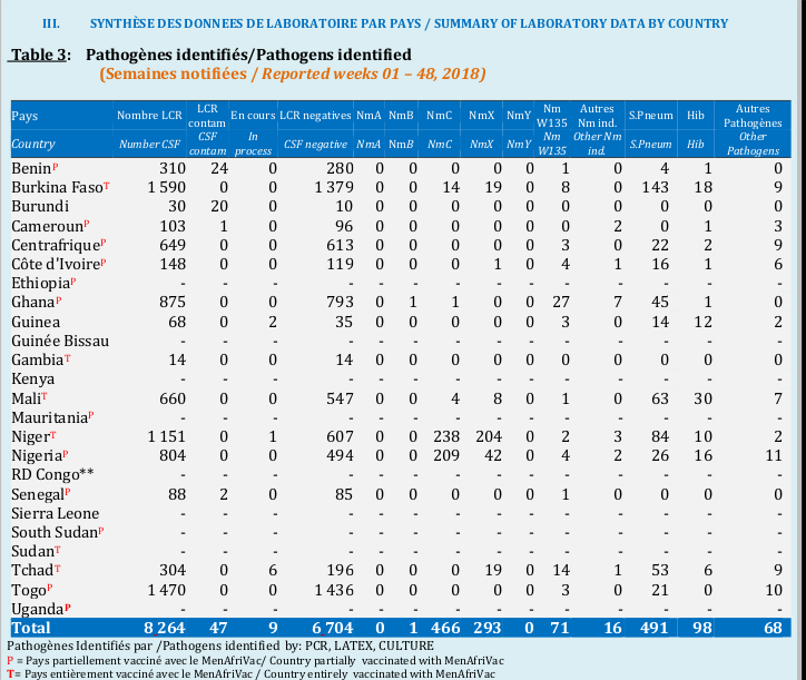
We will not go deeper in explaining the meaning of each column. We keep in mind that, at the end of our data management party -and it will be funny-, we want to have a kind of similar table, with these new column names that matches columns in the table presented above:

• countries , number_csf

• csf_contam, in_process, csf_negative

• nma, nmb, nmc, nmx, nmy, nmw135

• other_nm, s_pneum hib other_pathogens

Part one: extracting the row data

Once you succeed installing the tabulizer package, the extracting part is fairly simple. The package has a function for it, extract_pdf which has as arguments the file name, the page where we want to extract the table, the desired method of extraction and the format we want to get as result. Assuming my PDF is in the data folder we can write this:

pathogen_data <- extract_tables(
  #the pdf file path
  file = "data/meningitis-bulletin-s44-48-2018.pdf",
  #the page where to extract the data. Remember, page 5.
  page = 5,
  #the output format
  output = "data.frame",
  #the method
  method = "stream"
)

About the output format

Once I launched the function extract_table, I thought we would have as final output a data.frame of the table in page 5. But no.

class(pathogen_data)

## [1] "list"

The purpose behind is really understandable. If the page contains more than one table, all the tables of the page are compiled within a list where each table has the output format I told the function to hold in the parameters.

Also worth to mention, It would be really interesting to have a data-frame as output and not a matrix. Why? Because we are too busy to bother about pathogen_data[i+j-k, i-k+2] in the data management part. Instead, we will focus on how to deal with problems within our data-frame using the dplyr syntax. Take your broom and feel free to add your inputs in comments.

Planning what to do.

Now let’s take a look on the data-frame (the only table) we have in the list. It’s its first element.

pathogen_final_data <- pathogen_data[[1]]

summary(pathogen_final_data)

##       X                 X.1                X.2           
##  Length:36          Length:36          Length:36         
##  Class :character   Class :character   Class :character  
##  Mode  :character   Mode  :character   Mode  :character

A brief summary shows us only three variables in the data-frame, all characters and named respectively X, X.1 and X.2. We might want to have a global look on these three variables simultaneously, but I will move step by step since the data is really a mess. Let’s create a function which will print just one selected column of my data-frame pathogen_final_data. I want to access the column - which will be passed as a parameter- of my data in a way that should be understood by the select verb of dplyr, so I will put tidy evaluation in the game.

print_column <- function(.data, column, n_lines){
  #enquo to quote the parameter
  col <- enquo(column)
  .data %>% 
  #bang bang to unquote
  select(!!col) %>% 
  #print the number of lines
  head(n = n_lines)  %>% 
  datatable(class = "cell-border stripe",
            option = list(
            compact = TRUE,
            pageLength = 6,
            scrollX = TRUE),
            rownames = FALSE)
}

#It is a really mess, the first column
pathogen_final_data %>% 
  print_column(X, n_lines = 17)

It seems that we have the countries are in the column named X. This column has incorporated the section title and the name of the table. Also, we have some T and P at the end of the country names and we might have some encoding issues as you can see with one country Cote d'Ivoire in the table. There is also some blank lines at the beginning of the table.

What about the second column?

#It is more messy the second column
pathogen_final_data %>% 
  print_column(X.1, n_lines = 12)

Oops! We have a lot of empty lines at the beginning of the column. The columns of my final data-frame I have in mind as output seem to be merged together.

The third one?

pathogen_final_data %>% 
  print_column(X.2, n_lines = 13)

OK. We even don’t know what is in this data-frame. Fortunately, We have the table’s look in the report. So here are what we are expected to do ²:

• Split the columns so that we can have the data separated

• Remove the empty lines at the top of the data-frame.

• Remove the T and P at the end of country names.

• Give meaningful column names to my data and convert to the correct type each column.

In this post, we are only going to focus on the first part.

Defining some little things

countries_names <- c('uganda',        'togo',          'tchad',        
                     'sudan',         'south sudan',   'sierra leone', 
                     'senegal',       'rd congo',      'nigeria',
                     'niger',         'mauritania',    'mali',
                     'kenya',         'gambia',        'guinee bissau',
                     'guinea',        'ghana',         'ethiopia',
                     "cote d'ivoire", 'centrafrique',  'cameroun',
                     'burundi',       'burkina faso',  'benin',
                     'tanzania')

#creating the final column heading
final_columns <- c("countries",  "number_csf",   "csf_contam",
                   "in_process",  "csf_negative", "nma",
                   "nmb",         "nmc",          "nmx",
                   "nmy",         "nmw35",        "other_nm",
                   "s_pneum",     "hib",          "other_pathogens")

#find the percentage of empty values in a column
#vect is a character vector
percent_empty <- function(vect) sum(vect == ""| vect == "-") / length(vect)

#basically, the function can work with every data type, but let's consider
#only data-frame. The Threshold is exclusive

filter_empty_column <- function(.data, threshold = 1){
  
  #filter in the data.frame, columns where the percentage
  #of empty values is bellow the threshold.
  
  Filter( function(x) (percent_empty(x) < threshold), .data)
}

#start will help indexing the begining of 
#columns (either 0 or a given digit)
rename_columns <- function(.data, start = 0L){
  
  #Getting the number of columns from the data-frame
  nb_cols <- seq_along(colnames(.data)) + start
  
  #Changing the column names
  if( length(nb_cols) == 0L ){
    
    #stop with empty data, to let me check where the error
    #comes from
    stop("no colnames found")
  }
  else{
    colnames(.data) <- paste("columns", nb_cols, sep = "_")
    
  #returning the data frame. 
  .data
  }
}

#let'us take a look on an example dataset
mtcars %>% 
  as_tibble() %>% 
  rename_columns() %>% 
  print_column(everything(), n_line = 2)

Splitting the columns and correcting the country names

Since the separator for merged columns is the space character, what will be interesting is to split every column in the data-frame. As we are planning to clean the country names , we will keep the first column when splitting.

#function for splitting a vector and returning a tibble
split_vector <- function(vect){
  str_split(vect, "\\s", simplify = TRUE) %>% 
    as_tibble()
}

# a function to split the data

split_columns <- function(.data){
  
  #first, renaming the columns of my data
  .data <- rename_columns(.data)
  
  #second, stock the first column somewhere
  first_column <- .data %>% 
    select(columns_1)
  
  #third, split all columns of the data.frame
  splitted_data <- .data %>% 
    #using the purr package here
    map_dfc(split_vector) 

first_column
#finally, bind columns by including the first column
 first_column %>%
    bind_cols(splitted_data) %>%
    #rename columns to be sure about the final output
    rename_columns()
}

In the writing process we will have to take a regular look on our data set. To avoid copy-pasting, we are going to create a little function to print the data-frame.

#function to print the pathogen_final_data

have_a_look <- function(){
  pathogen_final_data %>% 
  print_column(columns_1:columns_10, n_lines = 10)
}

#splitting
pathogen_final_data <- split_columns(pathogen_final_data)
#printing

have_a_look()

We learnt how to split all columns of a data-frame and keep the first column within the final output and a use case of quotation.

In the next Step, we will deal with the three remaining problems.